Detecting potholes on roads from camera images can be beneficial for safe driving and also road maintenance planning. In this project we will explore this possibility using Deep Learning.
What are we building?
We are building a deep learning model using python code with Tensorflow API.
![]()

What can it do?
The model can take an image that contains road images (left image) and show us if there are potholes (right image) on it using blue colored splashes.

The output also prints out the collective pothole area percentage with respect to the total image.
How does it do it?
The model uses a technique which is popularly known as Instance Segmentation in computer vision. It also uses object detection technique along with that. This is possible by using the Mask RCNN algorithm.
This algorithm was developed by the Facebook AI Reasearch Team to do object detection and instance segmentation. To know everything with deeper understanding go to this link on github.
Object detection
Object detection is a technique that draws a rectangular box around an object and labels it with a predefined class and a confidence score. Example below:

For object detection the Mask RCNN algorithm relies on the Faster RCNN network which is in-built into the algorithm.
Instance Segmentation
This step isolates the pixels associated with each object into separate groups. Example:
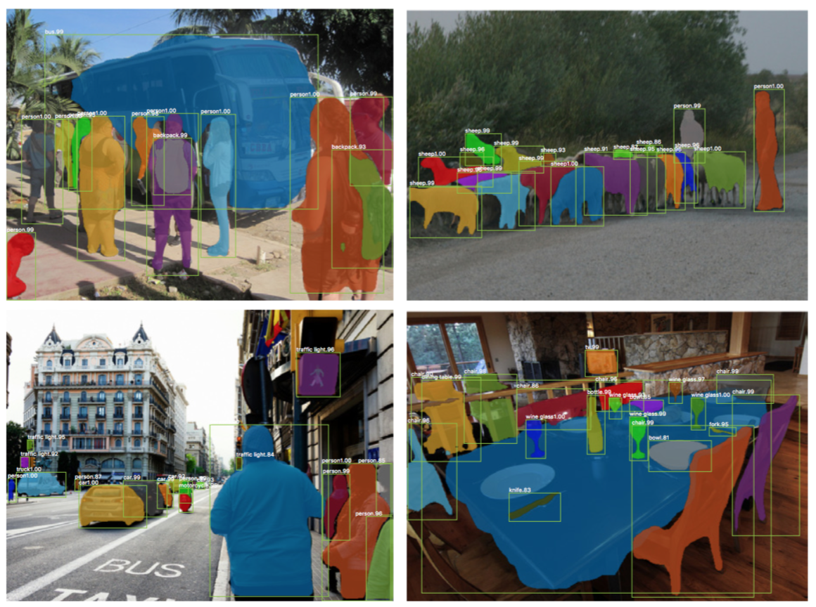
Image processing
After we get the pothole mask, we need to apply one more algorithm to get the color splash only on those spots. The code is defined in the pothole.py file and looks like following:
# =========================

# create a CLAHE object (Arguments are optional).
img_yuv = cv2.cvtColor(image, cv2.COLOR_BGR2YUV)


# convert the YUV image back to RGB format

clahe = cv2.createCLAHE(clipLimit=3.0, tileGridSize=(6,6))

# equalize the histogram of the Y channel
img_yuv[:,:,0] = clahe.apply(img_yuv[:,:,0])

img_yuv = cv2.cvtColor(img_yuv, cv2.COLOR_YUV2BGR)

hsv = cv2.cvtColor(img_yuv, cv2.COLOR_BGR2HSV)
blur = cv2.medianBlur(hsv,51)
mask_dry = cv2.inRange(blur,(0, 0, 0), (255, 255, 255))
overlay = image.copy()
outimg = image.copy()
# overlay[mask_dry==0] = (200, 80, 200)
overlay[mask_dry==0] = (10, 180, 200)
# overlay[mask_dry>0] = (10, 180, 200)

# apply the overlay
cv2.addWeighted(overlay, 0.5, img_yuv, 0.5, 0.8, outimg)
This piece of code extracts the pothole regions and colors them blue and also enhances the contrast of the final image.
How to build this?
To build a model that can work on our own images and objects, there are few steps we have to follow:
1. Collect pictures:
We need to collect as many pictures as possible that contain the objects we want to recognise. Usually, we can start by collecting few hundred images (say 200). In our specific case it is pictures of the roads which may contain potholes in a variety of ways. By ‘ways’ I meant the followings:
- different shapes of potholes
- there may not be not be wet at all
- pictures can be normal or cropped
- pictures are taken from different angles
- pictures are taken in various light and shadow conditions
- pictures are taken with different traffic situations
- potholes should have a clear boundary
2. Prepare the dataset
Now that we have the pictures, we have to prepare them for the algorithm.
To feed the images to the algorithm they have to go through the following process:
a) Divide the images into two sets:
We have to divide the images into two folders, namely train and val. A ratio of 80% training and 20% validation images is prefered.
b) Image annotation and labeling:
Image annotation is a process where we draw regions on the objects of our interest and label them accordingly.
To do this we make use of the image annotation tools. In our case we will be using the open source VIA tool provided by Oxford University. Download the app as shown below:

Then we extract the downloded file and open the via.html file
In this web app we can open all the images we want to train the model on.


In this web app we can open all the images we want to train the model on.

Then draw regions on them and also specify a class name. So, we open all the images and create a class named “pothole”.

We the start by drawing a polygon on the first image, surrounding the pothole. We draw multiple regions for multiple potholes. An example is shown below:

We then draw regions on all the images and click on save project icon. A json file will be downloaded by the browser. We need to copy this file to the images folder and rename it to via_region_data.json.
We need to do this process for both of the image sets separately.
3. Train the model
By now we should have a dataset directory like this:
 |-dataset
 | |-train
 | | |-1.jpg
 ...
 | | |-via_region_data.json
 | |-val
 | | |-1.jpg
 ...
 | | |-via_region_data.json
Install conda from this link if not already installed.
Now we clone the github repo: https://github.com/Rajat-Roy/potholes
git clone https://github.com/Rajat-Roy/potholes.gitnavigate into the code folder:
cd potholesTo start a conda environment execute:
conda create --name pothole python=3.7conda activate pothole
install dependencies:
pip install -r requirements.txtNow copy the dataset directory into this directory.
To start training execute the following command:
python train_model.py train --dataset=./dataset/ --weights=cocomodel training will now start and print the progress…
after the model training completes we will have a model file inside the logs directory named :
mask_rcnn_pothole_0030.h5Copy this file to the code root directory.
If model training stops for any reason we can resume it by running this command:
python train_model.py train --dataset=./dataset/ --weights=last
Congratulations! Model training is complete.
How to run this?
To run on Google Colab with zero setup, open this notebook and follow the instructions on the notebook.

You can just press Ctrl+F9 to run all the cells at once and scroll down to see the outputs like below once execution is completed without doing anything else.

We can run the code on new image within the jupyter notebook. Execute the following code in the conda prompt to open it:
jupyter notebookA jupyter app will open in the browser. Click on the file named pothole_demo.ipynb. The notebook will open. Make sure the file names and paths are correct. Run all the code cells from the menu option or press alt+Enter to execute cell by cell. You will see a result like this:
Total image area: 500x800 pixelspothole area: 7.76% (blue)
Congratulations again on running the first test.
Now you can keep on testing on other images by changing the filename in the last code cell and running only that cell.
Are the results accurate?
The results depend on the variety of pothole images it was fed during training.
In general it can give quite accurate results most of the time.
In future, I would like to differentiate the types of potholes and define different classes for them. I believe it will improve the performance of the model because it will not be confused to tackle all the varieties of potholes into a single class.